| Matrix scoring and alignment method |
Q3 accuracy (%) |
| BLOSUM62 profile CLUSTALW |
70.8 |
| Frequency profile CLUSTALW |
71.6 |
| Frequency profile PSIBLAST |
72.1 |
| HMMER Profile CLUSTALW |
74.4 |
| HMMER Profile Iterative Alignment (see Figure 2) |
74.3 |
| PSSM PSIBLAST |
75.2 |
| Numerical average of HMMER and PSSM PSIBLAST |
76.5 |
| Jury/No Jury network (see Figures 3 and 1) |
76.9 |
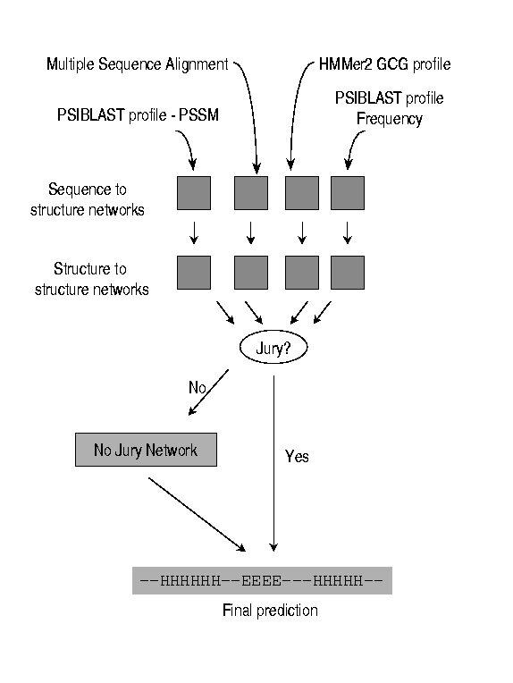
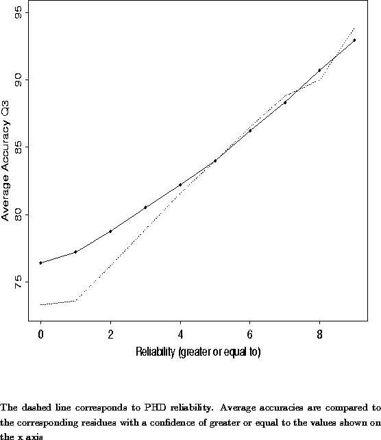
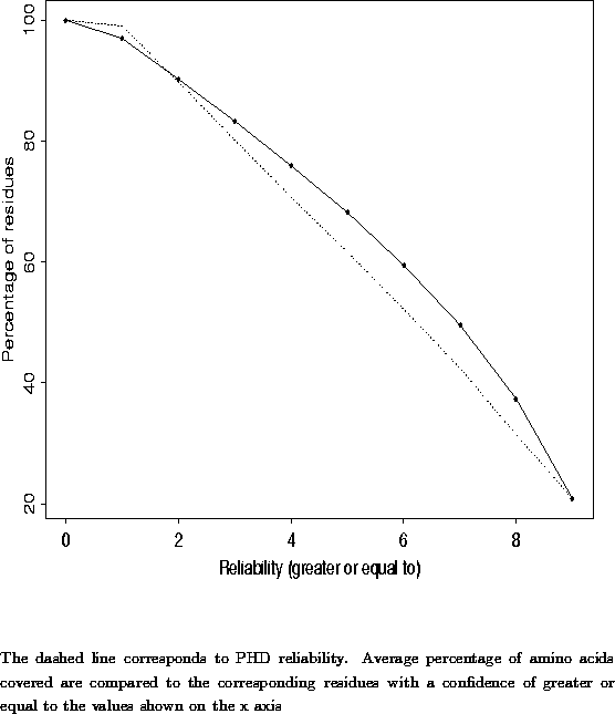
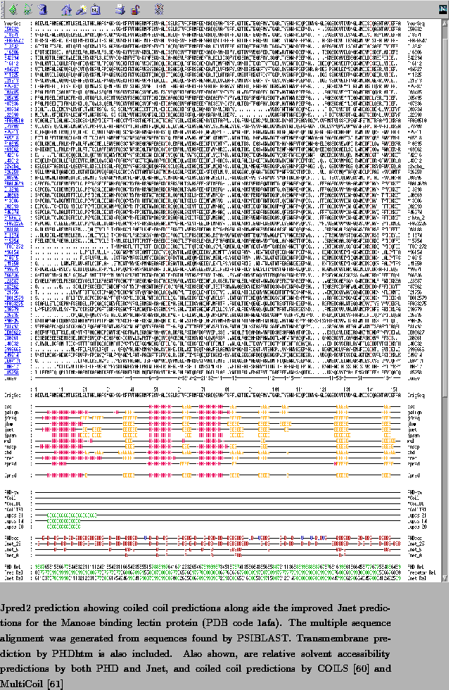
![\begin{landscape}% latex2html id marker 226
\begin{figure}[h]
\begin{center}
\le...
...ed proteins from a profile based search.}\end{center}\end{figure}\end{landscape}](img7.png)