


Smith and Waterman [Smith & Waterman, 1981] identified the best local alignment by
storing the entire H matrix, finding the maximum element, then
tracing back through the matrix. Waterman and Eggert
[Waterman & Eggert, 1987] described an algorithm to identify alternative locally optimal
alignments by partial re-calculation of the H matrix subject to the
condition that the alignment paths do not intersect, and that the
first and last equivalenced pairs have a positive score. Here, I show
that for a length-dependent gap-penalty the scores for all such
locally optimal alignments can be obtained on a single pass through
H. The essential observation is that since alignment paths are not
allowed to intersect, it is only possible to have one path passing
through each cell  . Therefore, when processing H it is
simply necessary to maintain a record of the starting residues and
best score for the alignment that passes throught the current cell
. Therefore, when processing H it is
simply necessary to maintain a record of the starting residues and
best score for the alignment that passes throught the current cell
 . The algorithm requires storage for the column scores C
as for the single best score algorithm. In addition, the current
maximum path scores M, and the start and end of the local alignment,
S, E, where S and E hold the co-ordinates of the cells in H
where the alignment starts and ends must also be stored.
. The algorithm requires storage for the column scores C
as for the single best score algorithm. In addition, the current
maximum path scores M, and the start and end of the local alignment,
S, E, where S and E hold the co-ordinates of the cells in H
where the alignment starts and ends must also be stored.
Figure 2(a-i) illustrates the processing of H to find the first, but
not the highest scoring, locally optimal alignment between the
sequences. For the sake of clarity, only the elements of C, M,
S and E that are relevant to this alignment are illustrated in
each figure. Figure 2a shows the first cell in the alignment
 , this is also the maximum score for the alignment so far,
and the alignment starts and ends with the same pair of residues
, this is also the maximum score for the alignment so far,
and the alignment starts and ends with the same pair of residues
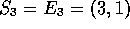 . In Figure 2b, the alignment is continued,
but since the current cell,
. In Figure 2b, the alignment is continued,
but since the current cell, 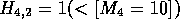 ,
,  ,
,
 and
and  are left unchanged. In Figure 2c,
  ,
so
,
so  and
and  are updated to 11 and (5,3) respectively.
Similar processing is shown in Figure 2(d-e) where C, M, S and
E are updated to the values 12, 21, (3,1), (6,4), while
Figure 2f
illustrates termination of the path when
are updated to 11 and (5,3) respectively.
Similar processing is shown in Figure 2(d-e) where C, M, S and
E are updated to the values 12, 21, (3,1), (6,4), while
Figure 2f
illustrates termination of the path when  . Now that this
local alignment path has decayed to zero, the starting and ending
coordinates are saved together with the alignment score. However,
since we have not completed the processing of H, we do not yet
know if this is the best possible score for an alignment starting in
. Now that this
local alignment path has decayed to zero, the starting and ending
coordinates are saved together with the alignment score. However,
since we have not completed the processing of H, we do not yet
know if this is the best possible score for an alignment starting in  .
Figures 2f-i, show that the alignment cannot be extended further, so
the maximum score of 21 for an alignment starting in
.
Figures 2f-i, show that the alignment cannot be extended further, so
the maximum score of 21 for an alignment starting in  stands.
Had it been possible for the alignment to be extended, then the new
best-score and end-point (M and E) would have replaced the 21,
(6,4) currently saved on the results list. Once the entire matrix has
been calculated (but not stored), the results list contains the score,
start and end co-ordinates for all local alignments between the two
sequences. Although not essential for the functioning of the
algorithm, it is often desirable to set a minimum score threshold
stands.
Had it been possible for the alignment to be extended, then the new
best-score and end-point (M and E) would have replaced the 21,
(6,4) currently saved on the results list. Once the entire matrix has
been calculated (but not stored), the results list contains the score,
start and end co-ordinates for all local alignments between the two
sequences. Although not essential for the functioning of the
algorithm, it is often desirable to set a minimum score threshold
 such that only those local alignments where
  will
be saved on the results list.
will
be saved on the results list.
If it is necessary to generate the alignments rather than just report
the best scores and end-points, then a direction matrix  [Smith et al., 1981,Gotoh, 1982] is saved during the calculation of H such
that each element
[Smith et al., 1981,Gotoh, 1982] is saved during the calculation of H such
that each element  indicates which of
 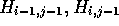 or
or  contributed to the value of
  . Accordingly,
 may be a compact data type of as few as 3-bits per element,
so the memory overhead for finding all locally optimal alignments
between long sequences is modest compared to algorithms that require
storage of H. Extension of the algorithm to allow gap-penalties of
the form
may be a compact data type of as few as 3-bits per element,
so the memory overhead for finding all locally optimal alignments
between long sequences is modest compared to algorithms that require
storage of H. Extension of the algorithm to allow gap-penalties of
the form  is straightforward if only best scores and
end-points are required, but generation of the corresponding
alignments will require two passes through H [Gotoh, 1982].
is straightforward if only best scores and
end-points are required, but generation of the corresponding
alignments will require two passes through H [Gotoh, 1982].
Figure 3 shows the 28 locally optimal alignments that are found
between the sequences A and B. Alignments of length 1
are normally uninteresting and so are excluded. The two
alignments illustrated by Waterman and Eggert [Waterman & Eggert, 1987] are ranked 1 and 2, with
a further six alignments scoring  . A total of 15 alignments
score
. A total of 15 alignments
score  with the remaining 13 optimal alignments scoring
 . Figure 4 illustrates the full H matrix with the
paths highlighted that correspond to the 15 alignments scoring
. Figure 4 illustrates the full H matrix with the
paths highlighted that correspond to the 15 alignments scoring  .
.